Still Matching Rows by Eye? XLOOKUP vs Power Query

01

You will recognise this

There is a list of orders and a list of customers. Or a list of invoices and a list of payments. Or timesheets and a staff roster. Two lists, sharing one thing in common, and the job is to bring a column from one across to the other.

So you open both, one on each screen. Read a reference number off the left. Find it on the right. Copy the value. Click back. Paste. Scroll. Repeat, four hundred times, while trying not to lose your place.

By row 250 you are working from muscle memory and you have stopped properly reading the reference numbers. That is not a criticism, it is what happens to everybody. It is also where the errors come from.

02

What it actually costs

The hours are obvious. These are the parts that are not.

• A pasted value looks identical to a correct one. A formula that finds nothing returns an error you can see. A human who pastes into the wrong row produces a number that looks completely normal and is wrong.
• The unmatched rows quietly disappear. When a reference has no partner in the other file, most people skip it and move on. Nobody ever goes back to the list of skipped ones, because there is no list.
• It cannot be spot checked. A reviewer would have to redo the whole thing to verify any of it, so nobody does, so it is never verified.
• The volume gets capped by the method. When someone asks for a full year instead of a month, the honest answer becomes no. The data was never the constraint.

The second one on that list is the one that costs real money. Unmatched rows are usually the interesting rows: the payment with no invoice, the order with no customer record, the timesheet entry against a project that closed.

03

Start with the formula, honestly

There is a version of this advice that jumps straight to the sophisticated answer. Ignore it. For a large share of these jobs, a lookup formula is the correct tool and takes ten minutes to learn.

XLOOKUP is the modern one. It searches a column for a value and returns whatever sits beside it, it can look left as well as right, and it lets you say what should appear when there is no match rather than leaving #N/A scattered through your work. We have a full walkthrough in our guide to using XLOOKUP in Excel, including the mistakes that produce most lookup errors.

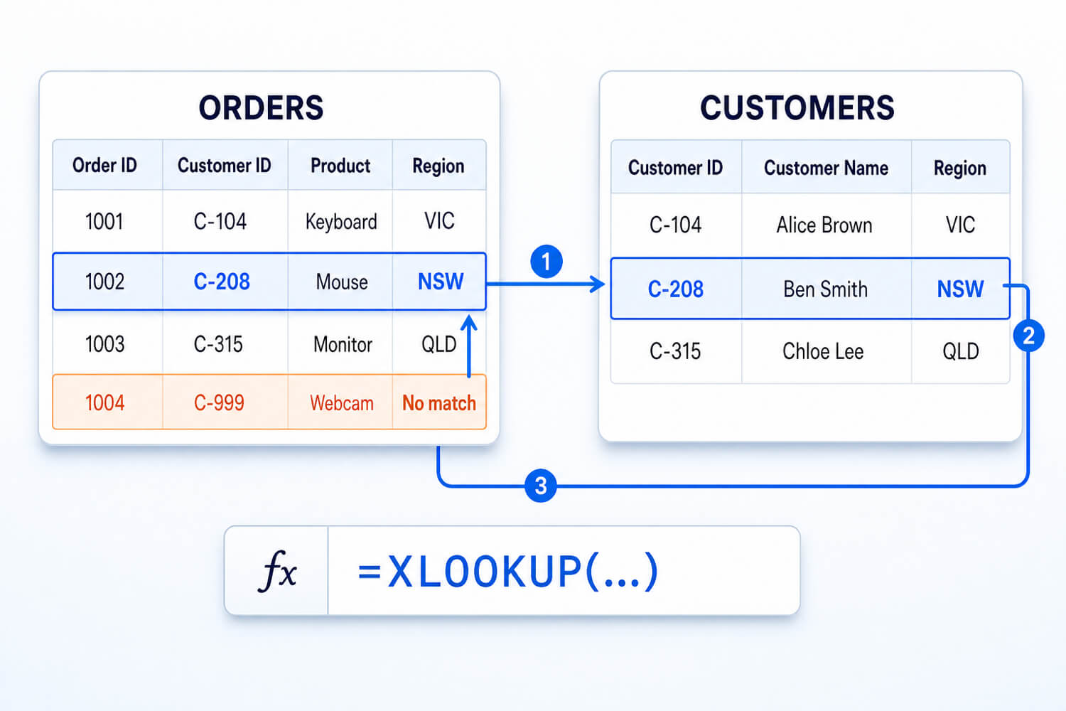
If you are still on VLOOKUP, the practical difference is maintainability. VLOOKUP often relies on a numbered return column, which can produce the wrong result when the structure changes. XLOOKUP points directly to the return column, making the formula easier to read and maintain.

04

The three signs you have outgrown it

A lookup formula has a ceiling. It is not about difficulty, and it is mostly not about size either.

Sign one: the other list is a separate file that arrives again next month. Formulas can link separate workbooks, but the process depends on file names, paths and ranges staying consistent. A refreshable query is usually easier to manage when the source keeps arriving again.

Sign two: you are matching on more than one column. Client name and month. Product code and region. A formula can do it, but it often needs a helper key or a harder-to-read compound formula. Merge lets you select several matching columns directly.

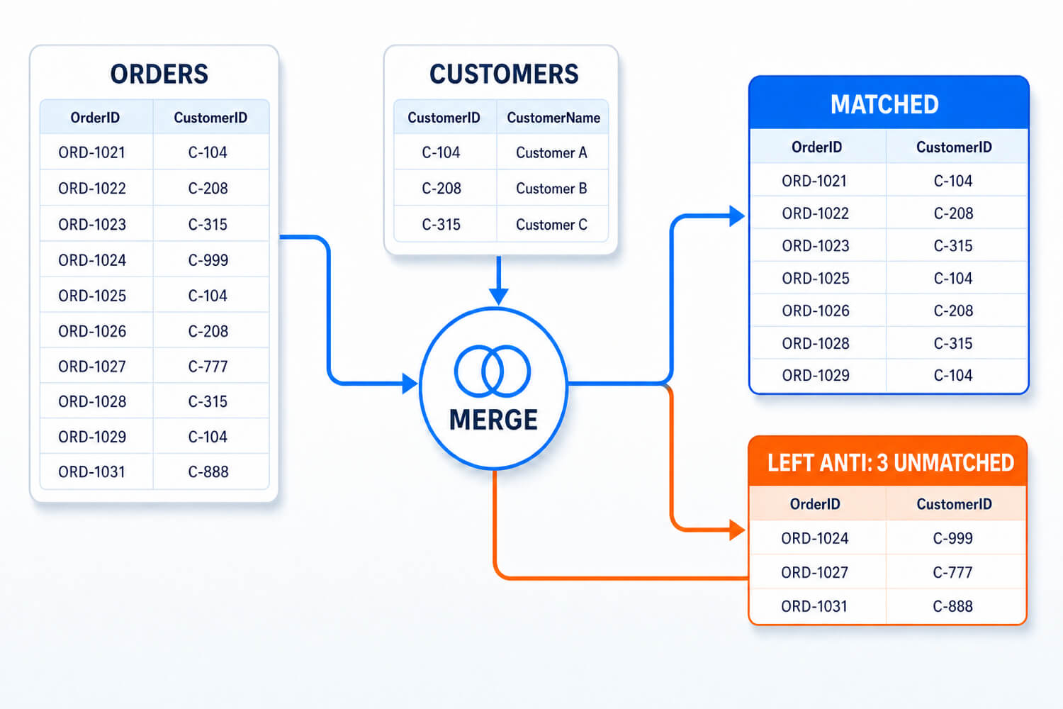
Sign three: you need to know what did not match. A lookup can flag a failed row, and additional formulas can produce a list of failures. A Left Anti merge makes that list a direct, refreshable output, which is usually easier for somebody to action.

Any one of those three is a good reason to consider Power Query's Merge. It joins two tables on one or several columns, and it lets you choose what to keep: everything from the left, only the rows that matched, or, and this is the useful one, only the rows that did not.

05

What it honestly takes to learn

• Around ten minutes to understand XLOOKUP on a clean pair of lists. This is genuinely a same-afternoon skill.
• A few guided hours to become comfortable with Merge, including the six join types and why "left outer" is the one you will use most often.
• The hard part is neither. It is noticing that two lists which look like they share a key actually do not, because one has trailing spaces, or stores the reference as text while the other stores it as a number. That is the skill, and it is the one an instructor saves you weeks on.

Excel Intermediate covers lookups and tables properly. Data Transformation using Power Query Editor covers merge, append and the cleaning that makes both keys line up in the first place.

Try this in ten minutes

Find out what does not match

Take copies of the two lists you usually reconcile by hand.

1. Put each list in its own sheet and turn both into Tables with Ctrl+T.
2. Click inside the first table, then Data, From Table or Range. In the editor, Close and Load To, Only Create Connection. Repeat for the second.
3. Data, Get Data, Combine Queries, Merge. Pick both queries and click the column they share in each.
4. In Join Kind choose Left Anti. Click OK, then Close and Load.

What lands in your workbook is every row from the first list with no partner in the second. For most people running this on real data for the first time, that list is not empty, and the contents are a genuine surprise. To bring matching values across instead, change Join Kind to Left Outer, then expand the new table column and select the fields you need.

Build the capability

Related Nexacu courses

Instructor led, one day, face to face across Australia or live online.

Whole team doing the same reconciliation? Corporate training can be run on your own two files.

Common questions

Frequently asked questions

Do this next

Run the Left Anti merge on the two files you reconcile most often. It takes ten minutes and it answers a question nobody in your organisation has asked out loud: how many rows have we been quietly skipping.