Conditional Formatting in Excel Intermediate

I’ve been conducting Excel Courses for Excel Consulting for a couple of years now. Excel Intermediate is our most frequently offered course. In that course, Conditional Formatting seems to be the most favourite topic for most groups that I’ve come across. It’s easy to see why because:

• It allows you to colour code your data based on predefined conditions e.g. anything above $100,000, turns the cell green
• It is dynamic i.e. even after defining your conditions, if the value changes, the colours will update automatically. In the above example, if the value fall below $100,000, the cell will no longer be green
• It is an efficient way of Data Visualization as it uses colour, cell background, font format etc. to convey additional meaning

I can go on and on regarding the benefits of Conditional Formatting but perhaps it deserves a separate blog. My focus in this blog is a specific way of using Conditional Formatting. It was an interesting question I got from a course participant:

How to apply Conditional Formatting on one column based on another?

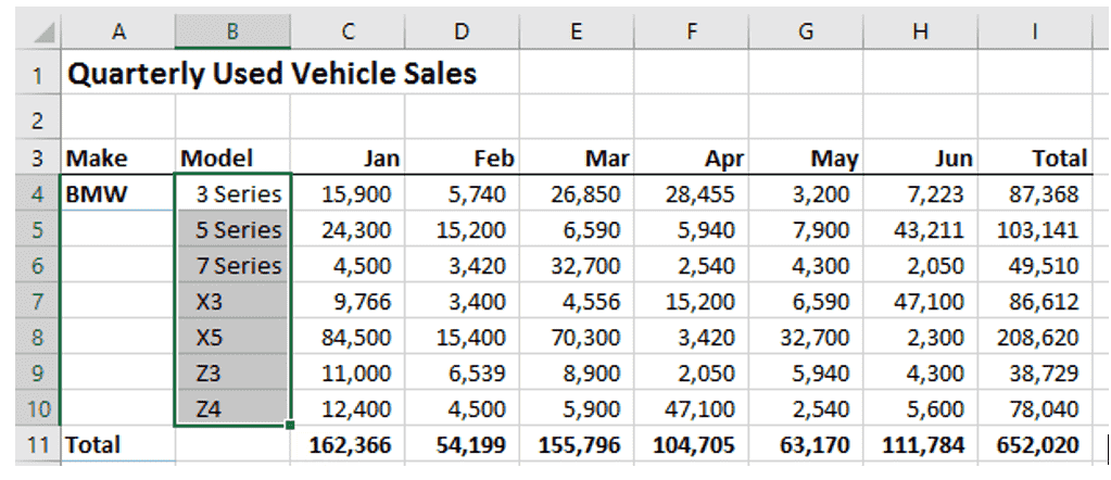
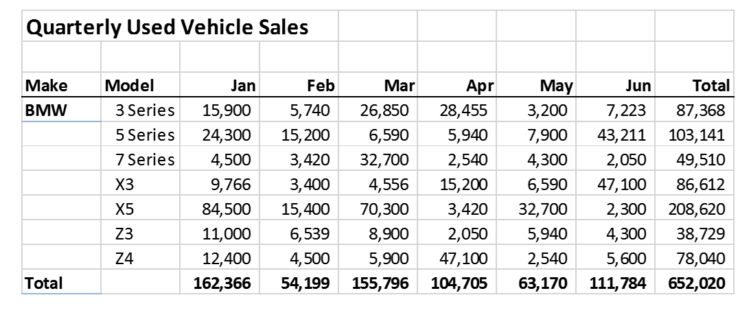
Let me try to answer that using an example. Let’s take the following data set:

Problem Statement:

The objective is to highlight the car Model based on the Total values e.g. if the Total is above $100,000, we want the respective car Model cell to turn green. Here’s how we do it:

Step 1:

Highlight the car Models


Step 2:

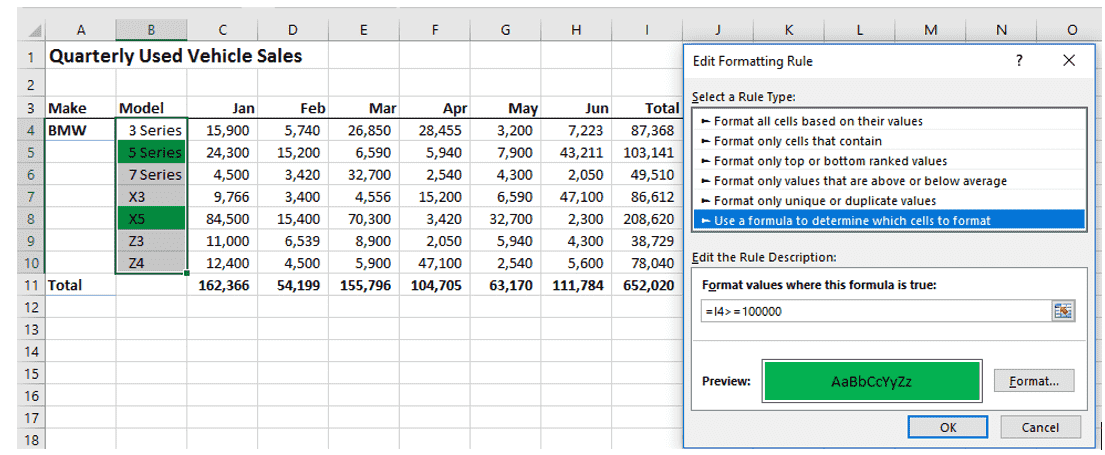
Go to Conditional Formatting -> New Rule -> Use a Formula to determine which cells to format

Step 3:

Type the following expression for the Formula: =I4>=100000 and then choose green Fill after clicking the Format button and then click OK. The Models above $100,000 ( 5 Series and X5) should turn green as a result.



I hope it’s a useful tip for those of you who want to explore Conditional Formatting and how it could be used in a specialized way.


Danny (Danish)

Learn how to effectively use conditional formatting (among other skills!) at our Excel courses.