Your guide to Pivot Tables

Pivot Tables are one of the most powerful tools in Excel. A Pivot Table is a table of statistics that summarises data from a more extensive table. They can be used to calculate, summarise and analyse data so you can interpret, report on and keep an eye on trends in your data.

Here’s a quick overview of how to create your own Pivot Table.

Step 1 - Enter your data in Excel

To create your Pivot Table, first you need to gather all your data in an Excel sheet so you can organise it.

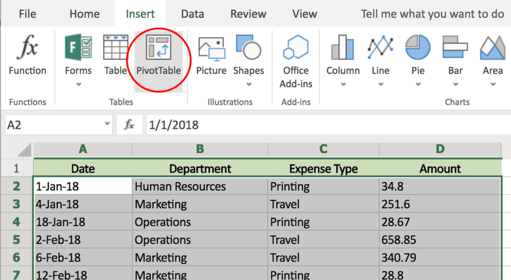
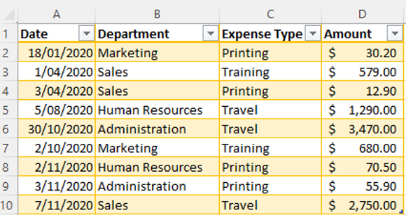
Enter all your values, ensuring you assign categories to your data in the topmost row or column, e.g. Date, Department, Expense Type and Amount.

This set of data shows types of expenses incurred from different departments in 2018.

To make it easier to interpret this dataset, we’d like to see how much each department spent in 2018 and on what type of expense.

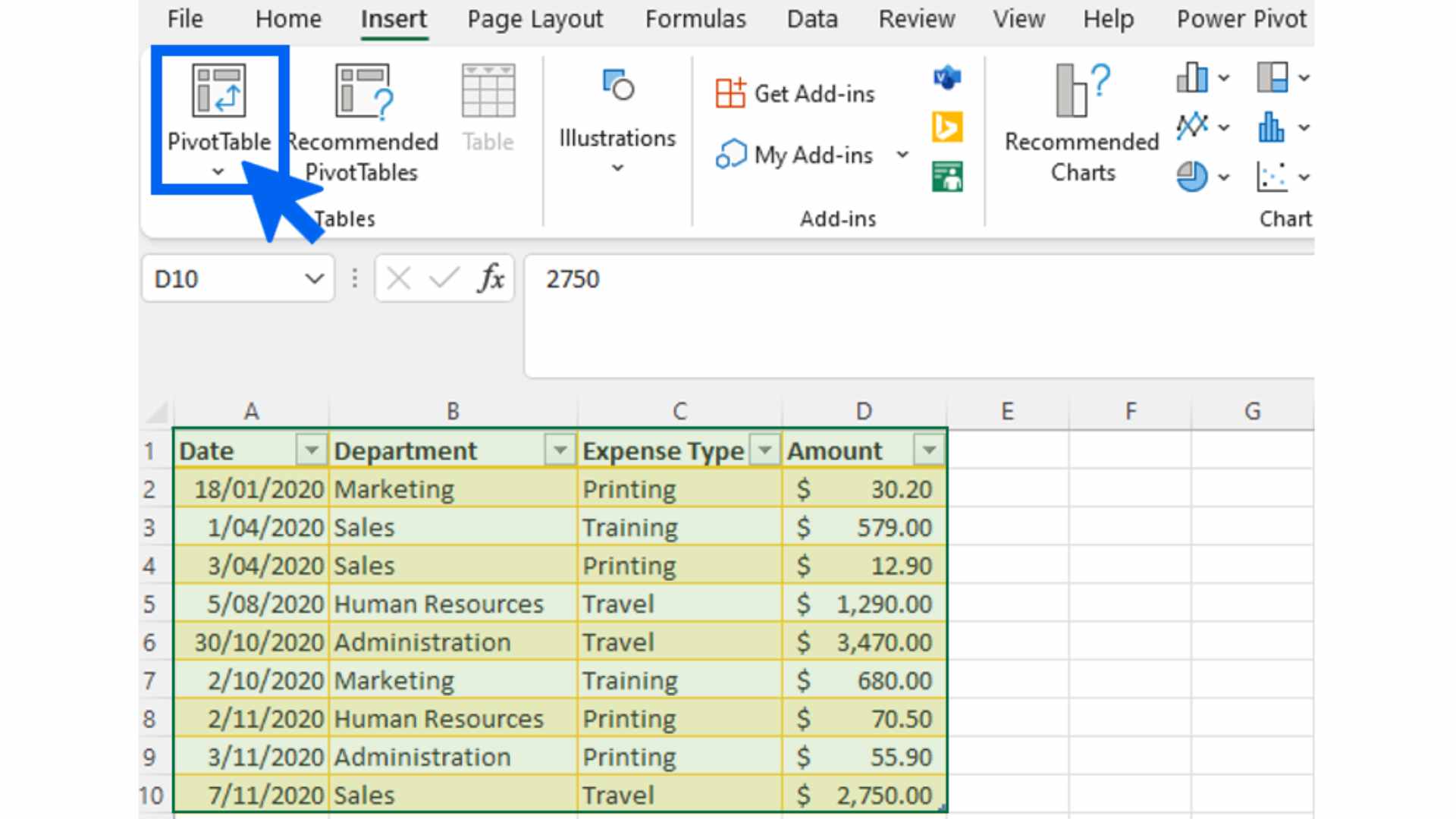
Step 2 - Select your data

To do this, select your data and then click Pivot Table under the Insert tab.

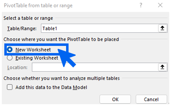
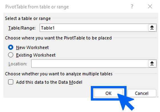
A pop-up dialogue will display. This allows you to choose where you want to place your new Pivot Table. We recommend selecting the "New Worksheet" option. Now click OK.

pivot table instructions

Step 3 - Customise your Pivot Table

A blank Pivot Table will be created. You can now customise how your data is summarised. This is easily done by dragging and dropping components to determine what identifier you’d like to organise your data by.

Let’s organise our set of data by department and expense, so we can see what the total of expenses were from each department.

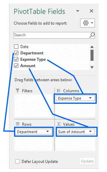
To do this, simply drag the Department field to the Rows box, then drag the Expense Type field to the Columns box, and finally drag the Amount field to the Values box.

And voila! You have created your first Pivot Table. We can now see at a glance, how much each Department spent and how they compare.

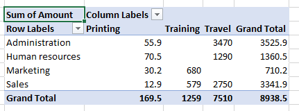
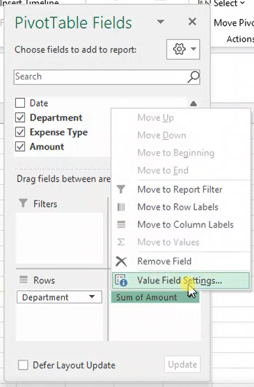
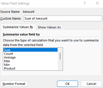
The Values column automatically calculates the Sum of Amounts as Grand Totals listed in your data. However, you can modify this Value column by clicking where it says "Sum of Amount". Then select Value Field Settings, and then select average, count or whatever field you need to apply to your data. The Pivot Table will update automatically.