
Conditional Formatting in Excel: Rules, Colour Scales & Data Bars Explained
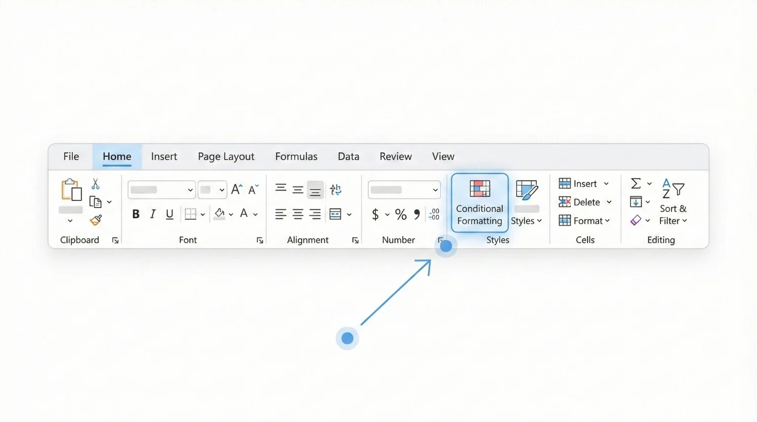
Conditional formatting lets you automatically colour cells based on their values so trends, outliers and issues are easier to spot at a glance. To get started, select your range and go to Home > Conditional Formatting, then choose a rule, colour scale or data bar.
In real AU/NZ workplaces, spreadsheets often become mini-systems: budgets, trackers, rosters, sales pipelines, service logs and reports that decision-makers rely on. Conditional formatting is one of the fastest ways to make those sheets clearer, safer and more readable without building charts or rewriting your workbook.
This guide explains the main types (rules, colour scales and data bars), shows you how to build a formula-based rule (the powerful bit), and shares practical tips for managing rules so your formatting doesn’t turn into an accidental rainbow.
TL;DR: Use Rules to flag exceptions (overdue, duplicates, missing data), Colour Scales for heatmaps (high/low patterns), and Data Bars for quick comparisons (progress or magnitude). For advanced needs, create a formula-based rule and manage rule priority in Manage Rules.
If your spreadsheet updates regularly, conditional formatting helps the sheet “self-police” so problems are visible before they become problems.
1) What is conditional formatting (and why use it)?
Conditional formatting is an Excel feature that changes the appearance of cells automatically based on rules you set for example, colouring overdue dates red, highlighting duplicates, or showing progress bars inside cells.
The big win is that the formatting updates as your data changes. That makes it ideal for shared workbooks where values are constantly edited, appended or imported.
- Budgets and variance reports
- Project and task trackers (due dates)
- Data quality checks (blanks, duplicates)
- Dashboards for KPI visibility
- Less manual formatting and rework
- Fewer “missed” issues in long tables
- More readable reports for stakeholders
- Simple rules can prevent costly errors
2) Rules vs colour scales vs data bars: what’s the difference?
Excel offers several conditional formatting styles, but most business users get the best results from three: rules, colour scales and data bars.
Practical recommendation: Start with one clear rule (e.g. overdue = red), then add visual layers (colour scale or data bars) only if they support decision-making. When in doubt, clarity beats decoration.
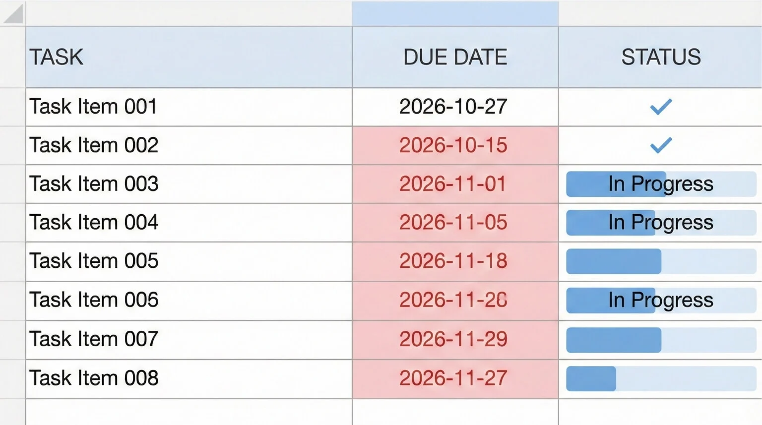
3) Rules: highlight what needs attention
Rules are the most direct type of conditional formatting. They’re ideal when you want Excel to “flag” cells or rows that meet a condition.
- Greater than / less than
- Between
- Text that contains
- A date occurring
- Duplicate values
- Top 10 items / Top 10%
- Bottom 10 items / Bottom 10%
- Above average
Tip: In small datasets, “Top 10” can be most of the table. Adjust the number so it stays meaningful.
- Select your due date cells (or the entire column of due dates).
- Go to Home > Conditional Formatting.
- Choose Highlight Cells Rules > A Date Occurring.
- Pick a date option (e.g. yesterday, last 7 days) and choose a format.
4) Colour scales: build a heatmap in seconds
Colour scales apply a gradient across a range, so high and low values stand out quickly. This is great for performance tables, budget variances, and KPI summaries.
- Select the values you want to compare.
- Home > Conditional Formatting > Colour Scales.
- Choose a 2-colour or 3-colour scale.
- When “higher” isn’t always “better” (e.g. stock on hand).
- When your range includes outliers that skew the gradient.
- When stakeholders interpret colours differently (keep it consistent).
For more control, go to Home > Conditional Formatting > Manage Rules and edit the rule to define custom minimum/midpoint/maximum settings (for example, based on targets rather than pure min/max).
5) Data bars: mini charts inside cells
Data bars are perfect for showing magnitude and progress without building a separate chart. They’re a favourite in operational reporting because they make long lists easier to scan.
- Select your numeric range (e.g. totals or % complete).
- Home > Conditional Formatting > Data Bars.
- Choose a style, then review the result.
Tip: In Manage Rules, you can enable Show Bar Only for a cleaner dashboard look.

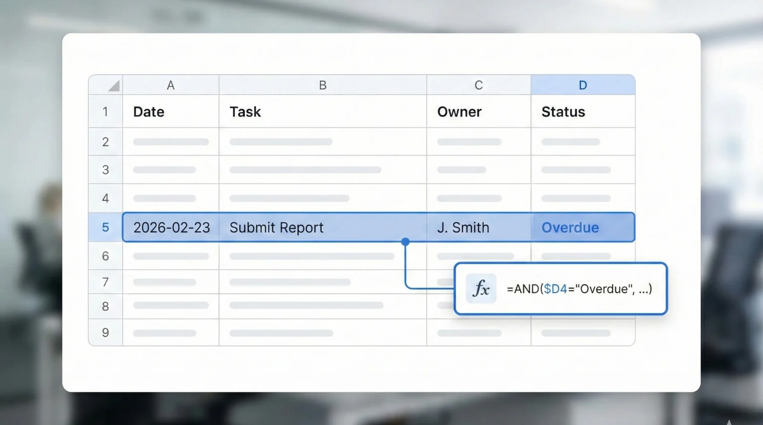
6) Formula-based rules: highlight rows, compare columns, and apply “business logic”
Formula-based rules are where conditional formatting becomes genuinely powerful. You can apply formatting based on another column, highlight entire rows, or build logic that mirrors your business process (without changing the underlying data).
Example setup: Column C contains Status (e.g. On track, At risk, Overdue). Your table starts on row 2.
- Select the table range you want to format (e.g. A2:F200).
- Home > Conditional Formatting > New Rule.
- Select Use a formula to determine which cells to format.
- Enter this formula:
- Choose a format (e.g. a subtle fill colour) and click OK.
Why the $ matters: $C locks the column so Excel always checks Status, while the row number updates for each row in your selection.
7) Manage Rules: control range, priority and “Stop If True”
If conditional formatting ever behaves unexpectedly, the answer is almost always in Manage Rules. This is where you edit, reorder and troubleshoot.
- Confirm the Applies to range is correct.
- Reorder rules so the most important one runs first.
- Delete duplicates or legacy rules you no longer use.
Excel applies rules in order. Stop If True prevents lower rules from overriding higher-priority formatting. This is useful when you want “Overdue” to stay clearly flagged even if another rule would also format the same row.
8) Common mistakes (and how to avoid them)
- Wrong range: the rule is applied to the wrong cells. Fix it in Manage Rules under Applies to.
- Reference errors in formulas: lock columns with $ when applying to multiple columns.
- Too many rules: lots of overlapping rules make results unpredictable. Keep only what supports decisions.
- Formatting masks the data: use subtle fills and consistent patterns for dashboards and reports.
Conditional formatting is a core skill in workplace Excel especially when combined with tables, formulas and good data habits. Nexacu offers instructor-led Excel Intermediate training across Australia (in-person or remote), where you practise conditional formatting in realistic reporting and tracking scenarios and learn how to build rules that stay reliable in shared files.
9) FAQs (expand to read)
These are common questions that come up in Excel training and internal support channels.
Does conditional formatting slow Excel down?
It can, particularly with very large ranges, lots of rules, or formula-based rules. Keep the “Applies to” range tight, avoid unnecessary rules, and prefer simpler conditions when possible.
Can I copy conditional formatting to other cells?
Yes. Copy and paste normally, use Format Painter, or use Paste Special > Formats. If you’re copying a whole worksheet section, check that the “Applies to” ranges still make sense afterwards.
Why does my formatting stop working when I insert rows?
Often the rule’s “Applies to” range didn’t expand. Converting your range to an Excel Table (Ctrl+T) is a reliable way to make rules expand as the table grows.
Can conditional formatting compare values across columns?
Yes. Use a formula-based rule (for example, comparing Actual vs Target) and apply it to the appropriate range. This is one of the most practical ways to build self-checking reports.
10) Next steps: make your sheets easier to trust
Conditional formatting is most effective when it supports a simple process: what needs attention, who acts, and when it’s considered resolved. A lightweight way to roll it out is to standardise a few rules in your team’s templates (for example: overdue, missing required fields, and above/below thresholds), then keep rules tidy using Manage Rules.
- Start small: one or two rules that prevent real mistakes (overdue, blanks, duplicates).
- Use tables: convert ranges to Excel Tables (Ctrl+T) so rules expand automatically.
- Set priorities: reorder rules so the most important “alerts” win.
- Document intent: add a small note (“red = action required”) so stakeholders interpret colours correctly.
- Review monthly: remove rules that no longer add value.
Apply conditional formatting confidently in real workplace scenarios
Nexacu’s Excel Intermediate course covers conditional formatting alongside the table, formula and reporting skills that make spreadsheets more reliable in shared environments with practical exercises built around common workplace patterns.
- Excel training courses
Short courses from beginner to advanced
- Excel Intermediate
Reporting, tables, formulas and automation basics
Note: Excel menus and features can vary slightly by version. If you work across mixed Excel environments, test conditional formatting rules in shared templates before standardising.